Least Squares and Its Applications Beyond Linear Equations
The best approximate solution to a system of linear equations, and applications beyond linear equations.
The Question
Suppose we are solving a system of $m$ linear equations in $n$ unknowns. We write the equations as $Ax=b$, where $A\in\R^{m,n},b\in\R^m$.
\[\left\{\begin{align*} A_{1,1}x_1&+A_{1,2}x_2&+\cdots&+A_{1,n}x_n&=b_1,\\ A_{2,1}x_1&+A_{2,2}x_2&+\cdots&+A_{2,n}x_n&=b_2,\\ &&&\vdots\\ A_{m,1}x_1&+A_{m,2}x_2&+\cdots&+A_{m,n}x_n&=b_m. \end{align*}\right.\]The textbook tells us to perform Gaussian elimination on the augmented matrix $\begin{bmatrix}A&b\end{bmatrix}$. The resulted row echelon form tells us whether the system has a solution and what the solutions are. However, when no exact solutions exist, sometimes we still want a “best approximate” solution, and this time Gaussian elimination cannot help.
To proceed, we must make precise the notion of a “best approximate solution”. The solution $x^*$ we seek is optimal in two senses.
- $x^*$ should minimize the mean squared error (MSE) $\frac1m\norm{Ax-b}^2$ (this loss function is self-explanatory and intuitive). Equivalently, $x^*$ minimizes $\norm{Ax-b}$. We call an $\hat x$ that minimizes the MSE a least-squares solution.
- However, the least-squares solution may not be unique. Let $\hat x$ be one least-squares solution. If the kernel of $A$ is nontrivial, then for any $x_0\in\ker A$, $\hat x+x_0$ also minimizes the MSE. Our desired solution $x^*$ should be a least-squares solution with minimal norm. Note that $x^*$ still may not be unique (e.g., when $A$ has two identical columns).
In short, we are searching for $x^*\in\R^n$ such that
Preliminaries
For our problem, some abstraction makes the picture clearer, and allows for further and more intriguing applications beyond solving linear equations.
Inner Product Spaces
For most of the time (almost always), you can think of a finite-dimensional inner product space as $\F^n$ with the Euclidean inner product. Doing so removes unnecessary complication and simplifies your thoughts.
Let $\F$ denote $\R$ or $\C$. An inner product space is a vector space $V$ over $\F$ along with a function (called inner product) $\inp\cdot\cdot:V\times V\to\F$ that satisfies the following axioms.
- Positivity: $\forall v\in V,\inp vv\geq0$.
- Definiteness: $\inp vv=0\iff v=0$.
- Linearity in first slot: $\inp\cdot v\in\L(V,\F)$ for each $v\in V$.
- Conjugate symmetry: $\inp vw=\overline{\inp wv}$ for every $v,w\in V$.
When we talk about $\F^n$, we tacitly treat it as an inner product space with the Euclidean inner product. For the rest of the article, suppose $V,W$ are finite-dimensional inner product spaces. We slightly abuse notation by using the same notation $\inp\cdot\cdot$ for inner products in different spaces.
Some examples of inner products are listed below to make the abstract definition more concrete.
\[\inp{(w_1,\dots,w_n)}{(z_1,\dots,z_n)}=c_1w_1\overline{z_1}+\cdots+c_nw_n\overline{z_n}.\]
- Suppose $c_1,\dots,c_n\in\R^+$. $\F^n$ is an inner product space with respect to
\[\inp fg=\int_{-1}^1fg.\]
- The vector space of continuous real-valued functions on $[-1,1]$ is an inner product space with respect to
\[\inp pq=\int_0^{+\infty}p(x)q(x)\e^{-x}\dx.\]
- The vector space of polynomials with real coeffcients is an inner product space with respect to
Suppose $e_1,\dots,e_n$ is an orthonormal basis of $V$. Then for any $v\in V$,
\[v=\inp v{e_1}e_1+\cdots+\inp v{e_n}e_n.\]$v$ is a linear combination of $e_1,\dots,e_n$. Applying $\inp\cdot{e_k}$ to both sides of $v=a_1e_1+\cdots+a_ne_n$ proves the theorem.
Orthogonal Projections
Recall that the Gram-Schmidt process (it holds mutatis mutandis for any (finite-dimensional) inner product space) transforms an independent list $v_1,\dots,v_m$ in $V$ to an orthonormal list $e_1,\dots,e_m$ with $\inp{v_k}{e_k}>0$ and $\spn(v_1,\dots,v_k)=\spn(e_1,\dots,e_k)$ for each $1\leq k\leq m$.1 The Gram-Schmidt process allows us to choose an orthonormal basis for a vector space, and to extend an orthonormal list to an orthonormal basis. We skip the proofs of some trivial results, which will be stated in the definitions.
For $U$ a subspace of $V$, the orthogonal complement of $U$, denoted by $U^\perp$, is defined as
\[U^\perp=\cbra{v\in V:\inp uv=0\text{ for all }u\in U}.\]- $U^\perp$ is a subspace of $V$.
- $\bra{U^\perp}^\perp=U$.
- $V=U\oplus U^\perp$.
We provide the proof sketch of the results above. Choose an orthonormal basis $v_1,\dots,v_m$ of $U$. Extend it to an orthonormal basis $v_1,\dots,v_n$ of $V$. It can be shown that $U^\perp=\spn(v_{m+1},\dots,v_n)$.
Now that $V=U\oplus U^\perp$, we can define the orthogonal projection operator.
Suppose $U$ is a subspace of $V$. The orthogonal projection operator onto $U$, often denoted by $P_U$, is defined as
\[P_U(u+w)=u\]for any $u\in U,w\in U^\perp$. The definition makes sense because every vector in $V$ can be written uniquely as the sum of a vector in $U$ and a vector in $U^\perp$.
Suppose $e_1,\dots,e_m$ is an orthonormal basis of $U$. Then
\[P_U(v)=\inp v{e_1}e_1+\cdots+\inp v{e_m}e_m.\]for any $v\in V$.
Extend $e_1,\dots,e_m$ to an orthonormal basis $e_1,\dots,e_n$ of $V$. Then
\[v=\inp v{e_1}e_1+\cdots+\inp v{e_m}e_m+\inp v{e_{m+1}}e_{m+1}+\cdots+\inp v{e_n}e_n\]for any $v\in V$. It can be verified that
\[\inp v{e_1}e_1+\cdots+\inp v{e_m}e_m\in U,\quad\inp v{e_{m+1}}e_{m+1}+\cdots+\inp v{e_n}e_n\in U^\perp.\]A Toy Answer
Let’s start from simple cases — real Euclidean spaces and matrices. We make the additional assumption that $A$ has independent columns, i.e., $\ker A=\{0\}$.
To minimize $\norm{Ax-b}$ is to find a vector in the column space of $A$ that is closest to $b$. Think of $\im A$ as a plane and $b$ as a point in $\R^3$. Geometry tells us that the error $b-A\hat x$ should be orthogonal to the plane (orthogonal to a basis of $\im A$). In other words, $A^\T(b-A\hat x)=0$. Hence
\[\hat x=(A^\T A)^{-1}A^\T b,\quad A\hat x=A(A^\T A)^{-1}A^\T b.\]Draw a picture yourself and you will understand everything in this section.
Following the intuition above, we give the rigorous proof.
Let $\hat x$ be the same as above.
\[\norm{b-Ax}=\norm{b-A\hat x-A(x-\hat x)}.\]$A^\T(b-A\hat x)=0$ leads to
\[\inp{A(x-\hat x)}{b-A\hat x}=(x-\hat x)^\T A^\T(b-A\hat x)=0.\]Hence the two terms are orthogonal. By the Pythagorean Theorem,
\[\norm{b-Ax}^2=\norm{b-A\hat x}^2+\norm{A(x-\hat x)}^2\geq\norm{b-A\hat x}^2.\]Note that $\ker A=\{0\}$. Hence the inequality is an equality if and only if $x=\hat x$. That implies that $\hat x$ is the unique least-squares solution.
When the columns of $A$ is linearly dependent ($\dim\ker A>0$), the method above obviously fails. That is why I call it a toy answer.
The Moore-Penrose Inverse: the Ultimate Weapon
Definition
The ultimate weapon is easier to understand in the context of linear maps instead of matrices (at least to me). We first give the definition.2
Suppose $T\in\L(V,W)$. The Moore-Penrose inverse, or pseudoinverse, of $T$ is a linear map from $W$ to $V$ defined as
\[T^\dagger=(\rest T{(\ker T)^\perp})^{-1}P_{\im T}.\]Note that $V=\ker T\oplus(\ker T)^\perp$. It can be shown that $TT^\dagger=P_{\im T}$ and $T^\dagger T=P_{(\ker T)^\perp}$.
A moment’s thought shows that $A^\dagger b$ is precisely what we are looking for.
- $A(A^\dagger b)=P_{\im A}b$. Hence $A^\dagger b$ minimizes the MSE.
- For any least-squares solution $\hat x$, $A\hat x=P_{\im A}b=A(A^\dagger b)$. Thus $\hat x=(\hat x-A^\dagger b)+A^\dagger b$, where the first term is in $\ker A$ and the second term is in $(\ker A)^\perp$ by definition. Hence $\norm{A^\dagger b}\leq\norm{\hat x}$ by the Pythagorean Theorem.
Calculation via Singular Value Decomposition
The definition of the pseudoinverse is obviously too computationally complicated to be practical. We show that the pseudoinverse can be calculated efficiently from the singular value decomposition (SVD).
I do not plan to prove the SVD in this article because it requires familiarity with too many prerequisites. I will state the theorem without proving it.
Suppose $T\in\L(V,W)$ and $s_1,\dots,s_m$ are the positive singular values of $T$. Then there exist orthonormal lists $e_1,\dots,e_m$ in $V$ and $f_1,\dots,f_m$ in $W$ such that for any $v\in V$,
\[Tv=s_1\inp v{e_1}f_1+\cdots+s_m\inp v{e_m}f_m.\]Equivalently, for $A\in\F^{m,n}$, there exist unitary matrices $U\in\F^{m,m}$ and $V\in\F^{n,n}$ such that
\[A=U\Sigma V^*,\]where $\Sigma\in\F^{m,n}$ is defined as
\[\Sigma_{j,k}=\left\{\begin{align*} \sigma_k&\quad,j=k\\ 0&\quad,\text{otherwise}. \end{align*}\right.\]Here the $\sigma$’s are the singular values of $A$.
The equivalence between the two forms can be shown by basic understanding of matrix multiplication. Because nice numerical techniques exist for computing the SVD of a matrix, the pseudoinverse can be calculated efficiently by the theorem below.
Suppose $T\in\L(V,W)$ and
\[Tv=s_1\inp v{e_1}f_1+\cdots+s_m\inp v{e_m}f_m\]is an SVD of $T$. Then for any $w\in W$,
\[T^\dagger w=\frac1{s_1}\inp w{f_1}e_1+\cdots+\frac1{s_m}\inp w{f_m}e_m.\]Equivalently, if $A=U\Sigma V^*$ is an SVD of $A\in\F^{m,n}$, then $A^+=V\Sigma^+U^*$, where $\Sigma^+\in\F^{n,m}$ is defined as
\[(\Sigma^+)_{j,k}=\left\{\begin{align*} \frac1{\sigma_k}&\quad,j=k\\ 0&\quad,\text{otherwise}. \end{align*}\right.\]We prove the linear map version of the result above. The proof contains some background knowledge about SVD which will not be introduced in this article. The matrix version follows from the definition of matrix multiplication.
Suppose $w\in W$. By some property of SVD, $f_1,\dots,f_m$ is an orthonormal basis of $\im T$. From the explicit expression of orthogonal projection operators (proved above),
\[P_{\im T}w=\inp w{f_1}f_1+\cdots+\inp w{f_m}f_m.\]It suffices to show that $T^\dagger f_k=\frac1{s_k}e_k$ for $1\leq k\leq m$. That follows from that $T(\frac1{s_k}e_k)=f_k$ and that $\frac1{s_k}e_k\in(\ker T)^\perp$ (a property of SVD).
Applications
Our abstraction of inner product spaces now enables us to work with vector spaces other than $\F^n$. Note that many results above hold as well in Hilbert spaces, but we do not talk about Hilbert spaces in this article and focus only on finite-dimensional cases.
I will only mention one example of the various applications. Suppose we are looking for a polynomial $p$ with real coefficients and degree no greater than $5$ that best approximates the sine function on $[-\pi,\pi]$. Here (suppose that) “best” is in terms of minimizing
\[\int_{-\pi}^\pi (p(x)-\sin x)^2\dx.\]We first make the vector space $C[-\pi,\pi]$ of continuous real-valued functions on $[-\pi,\pi]$ into an inner product space by defining
\[\inp fg=\int_{-\pi}^\pi fg\]for every $f,g\in C[-\pi,\pi]$. Let $\mathcal P_5(\R)$ be the subspace (of $C[-\pi,\pi]$) of polynomials with real coefficients and degree no greater than $5$. We are looking for $p\in\mathcal P_5(\R)$ that minimizes $\norm{p-\sin(\cdot)}$. That is equivalent to projecting the sine function onto the subspace $\mathcal P_5(\R)$.
We solve the problem with the explicit expression of orthogonal projection operators. First we perform the Gram-Schmidt process on the basis $1,x,\dots,x^5$ of $\mathcal P_5(\R)$. Mathematica tells me that the resulted orthonormal basis is3
\[\left\{\frac{1}{\sqrt{2 \pi }},\frac{\sqrt{\frac{3}{2}} x}{\pi ^{3/2}},\frac{3 \sqrt{\frac{5}{2}} x^2}{2 \pi ^{5/2}}-\frac{1}{2} \sqrt{\frac{5}{2 \pi }},\frac{5 \sqrt{\frac{7}{2}} x^3}{2 \pi ^{7/2}}-\frac{3 \sqrt{\frac{7}{2}} x}{2 \pi ^{3/2}},\frac{105 x^4}{8 \sqrt{2} \pi ^{9/2}}-\frac{45 x^2}{4 \sqrt{2} \pi ^{5/2}}+\frac{9}{8 \sqrt{2 \pi }},\frac{63 \sqrt{\frac{11}{2}} x^5}{8 \pi ^{11/2}}-\frac{35 \sqrt{\frac{11}{2}} x^3}{4 \pi ^{7/2}}+\frac{15 \sqrt{\frac{11}{2}} x}{8 \pi ^{3/2}}\right\}.\]Apply the explicit formula and we obtain the best approximation of the sine function
\[\frac{693 x^5}{8 \pi ^6}-\frac{72765 x^5}{8 \pi ^8}+\frac{654885 x^5}{8 \pi ^{10}}-\frac{315 x^3}{4 \pi ^4}+\frac{39375 x^3}{4 \pi ^6}-\frac{363825 x^3}{4 \pi ^8}+\frac{105 x}{8 \pi ^2}-\frac{16065 x}{8 \pi ^4}+\frac{155925 x}{8 \pi ^6}.\]It is numerically approximately equal to
\[0.987862 x - 0.155271 x^3 + 0.00564312 x^5.\]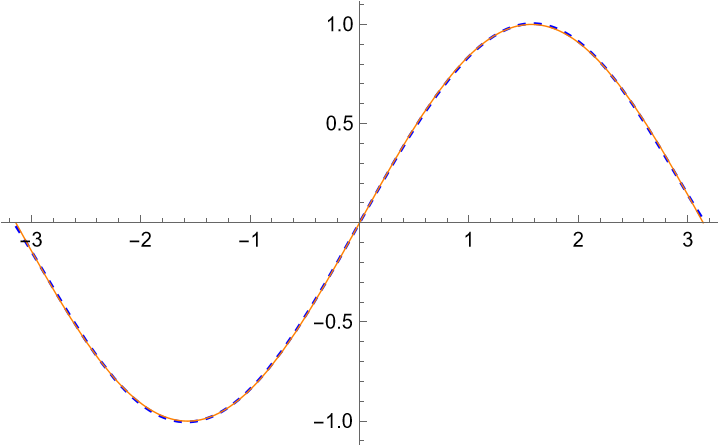 The orange solid line is the sine function, and the blue dashed line is our polynomial approximation.
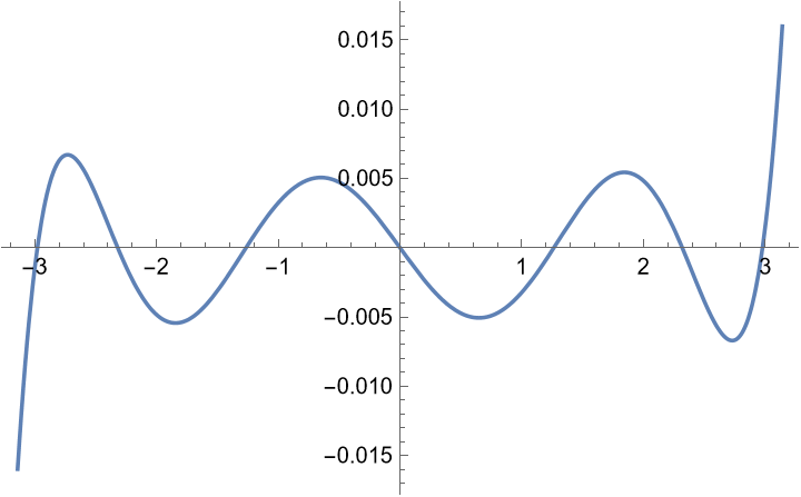 The error $p(x)-\sin x$.
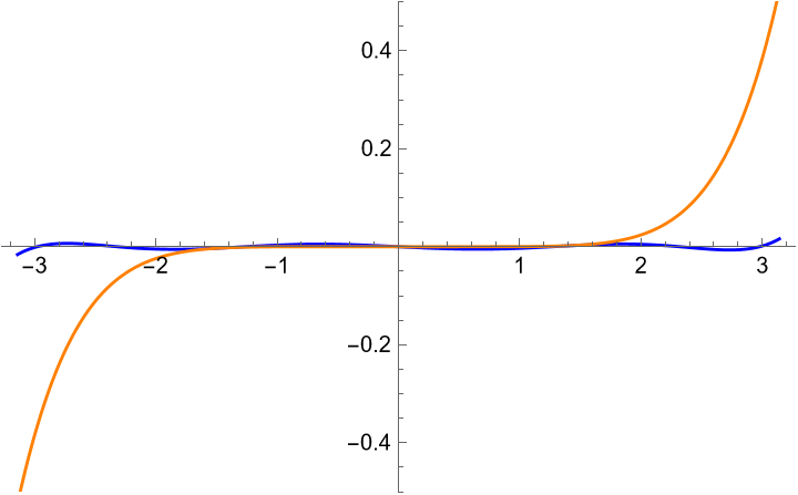 The blue line is the error of $p$, and the orange line is that of the Taylor polynomial.
If we project onto the subspace $\spn(1,\cos x,\dots,\cos nx,\sin x,\dots,\sin nx)$, the resulted best approximation is precisely the Fourier series. That is a very profound subject.